Chapter 2 — Regression
From data to linear prediction models
1 Chapter overview
Many questions in science and engineering involve estimating a numerical quantity from information that we can observe. We might estimate a person’s weight from height, predict sales from advertising expenditures, or forecast a bridge’s displacement from applied loads and measured conditions. Regression provides a framework for learning relationships between input variables and a numerical output. It can support both predictions for new observations and investigations of how an output varies with its inputs.
This chapter develops the regression problem and introduces linear regression as a particularly useful starting point. We establish the notation used to describe datasets, distinguish prediction from interpretation, and derive univariate and multivariate linear models. We then consider what it means to fit a model to data and why having more parameters than observations can make the fitted parameters non-unique. The final part reviews important qualifications, including correlation versus causation and the linear-algebra notation needed for subsequent chapters.
1.1 Learning objectives
By the end of the chapter, you should be able to:
- Explain the regression problem and distinguish its prediction and interpretation goals.
- Represent a regression dataset using input vectors, a data matrix, and a target vector.
- Recognize univariate and multivariate regression applications.
- Interpret the slope and intercept of a univariate linear regression model.
- Express multivariate linear regression using feature vectors, an intercept, and a dot product.
- Explain what parameter estimation or fitting aims to accomplish.
- Describe why an overparameterized linear model may have many equally good fits to the observed data.
- Distinguish association from causal effects and check basic matrix dimensions.
2 The regression problem
Regression studies the relationship between one or more input variables and a numerical output variable. Given observations of the inputs and the corresponding outputs, we aim to construct a function that approximates the output from the inputs. The function can then be evaluated for a new input or examined to understand relationships in the observed data. The important distinction from a classification task is that the output of an ordinary regression problem is a numerical quantity, not a class label.
Consider, for example, the relationship between a person’s height and weight. If height is known but weight is not, a regression model could estimate a plausible weight from height. In an engineering application, the input might instead be a measured load and the output a structural displacement. Real measurements generally contain variability: people of the same height need not have the same weight, and measurements of apparently similar structural systems may not coincide exactly. Consequently, we usually seek a function that predicts the output approximately, not one that reproduces every observation without error.
2.1 Representing a regression dataset
Suppose we have \(N\) observations, each with \(D\) input variables (also called features) and one numerical output (the target). We write the dataset as
\[ \mathcal D=\{(\mathbf x_n,y_n)\}_{n=1}^{N}, \qquad \mathbf x_n=\begin{bmatrix}x_{n1}&x_{n2}&\cdots&x_{nD}\end{bmatrix}^{\!\top}\in\mathbb R^D, \qquad y_n\in\mathbb R. \]
The index \(n=1,\ldots,N\) identifies the observation, whereas \(d=1,\ldots,D\) identifies a feature. The scalar \(x_{nd}\) is therefore the value of feature \(d\) for observation \(n\). \(N\) is the number of observations; \(D\) is the number of input features. These dimensions describe different properties of a dataset and need not be comparable in size. Depending on the application, either may be very large.
It is convenient to store all inputs in a data matrix \(X\) and all observed outputs in a target vector \(\mathbf y\):
\[ X=\begin{bmatrix} x_{11}&x_{12}&\cdots&x_{1D}\\ x_{21}&x_{22}&\cdots&x_{2D}\\ \vdots&\vdots&\ddots&\vdots\\ x_{N1}&x_{N2}&\cdots&x_{ND} \end{bmatrix}\in\mathbb R^{N\times D}, \qquad \mathbf y=\begin{bmatrix}y_1\\y_2\\\vdots\\y_N\end{bmatrix}\in\mathbb R^N. \]
Each row of \(X\) corresponds to one observation, and each column to one feature. The \(n\)th row is \(\mathbf x_n^\top\), and its output appears in the \(n\)th entry of \(\mathbf y\). This row-wise convention will make it possible to predict all \(N\) outputs with a single matrix multiplication later on.
| Observation | Feature 1: height (cm) | Feature 2: age (years) | Target: weight (kg) |
|---|---|---|---|
| 1 | 160 | 22 | 58 |
| 2 | 173 | 28 | 71 |
| 3 | 185 | 24 | 82 |
For this small, illustrative dataset, \(N=3\) and \(D=2\). For instance, \(\mathbf x_2=(173,28)^\top\) and \(y_2=71\). The matrix \(X\) has three rows and two columns, while \(\mathbf y\) has three entries. If only height were used, \(D\) would become 1 without changing \(N\). As in Chapter 1, the inputs do not need to come from conventional tables: pixels, numerical sensor measurements, and appropriately encoded text can also be organized into numerical features.
2.2 Examples of regression
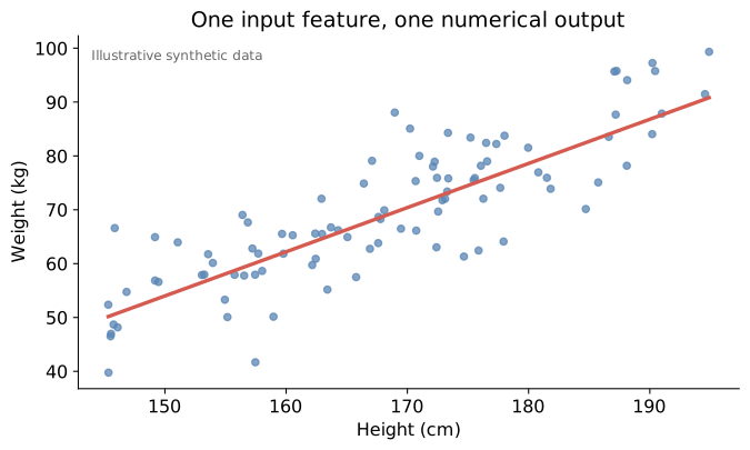
The height–weight relationship is an example of univariate regression, because only one feature is used to predict one numerical output. Each person gives a pair \((x_n,y_n)\), which can be plotted as a point in the plane. A visible trend suggests that height and weight are associated, although individual observations lie above or below any simple line. The presence of a trend does not tell us in advance whether a straight line is the best mathematical description; the data are observed first, and the model is chosen afterwards.
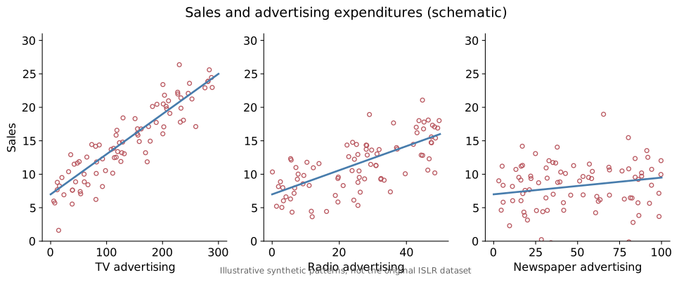
Regression also applies when several inputs are available. For example, a business may wish to estimate sales from expenditures on television, radio, and newspaper advertising. Each campaign then has three features, \(\mathbf x_n=(x_{n1},x_{n2},x_{n3})^\top\), and one output \(y_n\) representing sales. The strength of the relationship between sales and each individual advertising channel may differ; looking at three separate scatterplots is an informative starting point, but a single regression model can use the three inputs jointly.
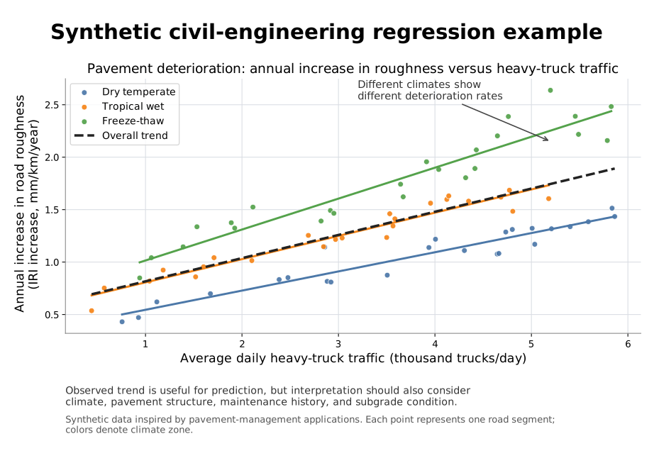
A more challenging civil-engineering example is the relationship between heavy-truck traffic and pavement deterioration. Suppose we study many road segments and relate the annual increase in pavement roughness to the average daily number of heavy trucks using the road. A regression model may reveal a clear positive trend: roads carrying more heavy vehicles often deteriorate faster. This relationship can be useful for prediction, for example when estimating future maintenance needs for a road with known traffic demand. However, the observed trend should not be interpreted in isolation. Pavement deterioration also depends on factors such as climate, pavement structure, drainage, construction quality, maintenance history, and subgrade condition. As a result, two roads with similar traffic volumes may still show different deterioration rates. This illustrates why regression is valuable for studying complex engineering relationships, while also emphasizing that careful interpretation requires attention to additional variables.
2.3 Prediction and interpretation: two distinct goals
Regression is commonly used for prediction and interpretation. In a prediction task, the aim is to estimate the output for an input whose output is unknown. For example, What is the predicted weight of a person who is 170 cm tall? Or What displacement should we expect under a particular load? The main concern is whether the model can make accurate predictions for new inputs.
In an interpretation task, the focus is on understanding how the output varies with one or more inputs. We may ask, Are taller people generally heavier? or How does the predicted structural displacement change as the applied load increases? These are questions about relationships, not merely about obtaining one numerical answer. A model may be useful for prediction without giving an easily interpretable explanation, and an apparent relationship may not have a causal meaning. Thus, high predictive accuracy and trustworthy interpretation are related but different objectives.
For both goals we introduce a regression function \(f\) and seek predictions
\[ \hat y_n=f(\mathbf x_n)\approx y_n, \qquad n=1,\ldots,N. \]
When the function is controlled by numerical parameters \(\mathbf w\), we make that dependence explicit:
\[ \boxed{\hat y_n=f_{\mathbf w}(\mathbf x_n)} \qquad or \qquad \boxed{\hat y_n=f_{\mathbf w}(\mathbf x_n, \mathbf w)} \]
Here, \(y_n\) is the observed output, \(\hat y_n\) is the predicted output, \(\mathbf x_n\) is the input, and \(\mathbf w\) describes the model. Choosing the form of \(f\) and determining suitable values for \(\mathbf w\) are two different decisions. We begin by choosing one of the simplest useful model families: linear regression.
3 Linear regression
Linear regression represents the predicted output as a linear combination of input features, usually with an additional constant term. It is an attractive first model because its parameters have clear meanings, its predictions are inexpensive to compute, and it provides a manageable setting for studying ideas shared with more complex learning methods. The model also provides a direct connection between mathematical functions and observed data.
3.1 Univariate linear regression: slope and intercept
When each input contains only one feature (\(D=1\)), we use the familiar equation of a straight line:
\[ \boxed{\hat y_n=f_{\mathbf w}(x_n)=w_0+w_1x_{n1}.} \]
The two parameters are \(\mathbf w=(w_0,w_1)^\top\). The intercept \(w_0\) specifies the model’s predicted value at \(x=0\), while the slope \(w_1\) describes the change in predicted output for a one-unit increase in the input. A positive slope corresponds to an increasing line; a negative slope corresponds to a decreasing line; and \(w_1=0\) gives a constant prediction. The units of the slope are the units of \(y\) divided by the units of \(x\).
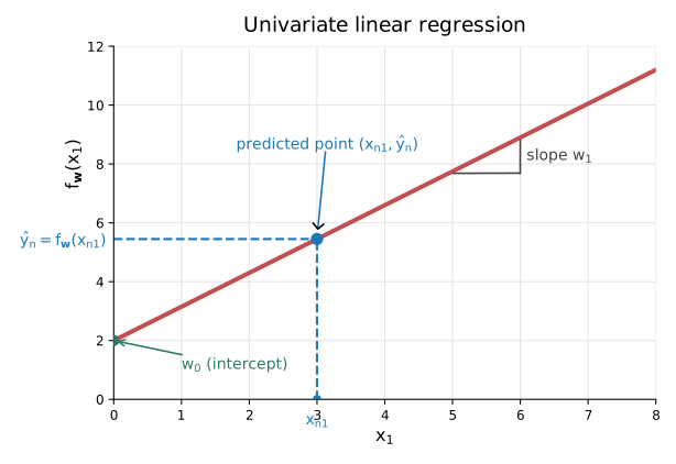
For a simple illustration, suppose a fitted model of displacement \(y\) (in mm) under load \(x\) (in kN) is \(f_{\mathbf w}(x_{n1})=1+0.4x_{n1}\). At a load of \(10\) kN, the predicted displacement is \(1+0.4(10)=5\) mm. The slope represents \(0.4\) mm/kN, meaning the model predicts an additional \(0.4\) mm of displacement for each additional kN within the conditions for which the model is appropriate. The intercept is a mathematical parameter; whether its value at zero load has a meaningful physical interpretation depends on the measurements and the problem. This relationship is a toy example, not a calibrated structural model.
When \(D=1\), the fitted model is a line in the \((x,y)\) plane. Its slope and intercept determine the position of that line. Observed points generally do not lie exactly on it because of variability, measurement noise, omitted factors, or imperfections in the chosen model. Fitting aims to select parameter values that make the differences between observations and predictions acceptably small according to a criterion introduced in the next chapter.
3.2 Multivariate linear regression: several features
When each observation contains \(D\) features, we generalize the straight line to a linear combination:
\[ \begin{aligned} \hat y_n=f_{\mathbf w}(\mathbf x_n) &=w_0+w_1x_{n1}+w_2x_{n2}+\cdots+w_Dx_{nD}\\ &=w_0+\sum_{d=1}^{D}w_dx_{nd}\\ &=w_0 + {\mathbf x}_n^\top{\mathbf w}. \end{aligned} \]
The parameter \(w_0\) is the intercept (also called the offset or bias term), and \(w_d\) is the coefficient associated with feature \(d\). There are \(D\) original input features but \(D+1\) model parameters when the intercept is included. This distinction matters when discussing how much information the dataset provides relative to the number of unknown parameters.
For two features, the prediction becomes \(\hat y_{n}=w_0+w_1x_{n1}+w_2x_{n2}\). Instead of a line, this expression describes a plane in a three-dimensional coordinate system with axes \(x_1\), \(x_2\), and \(y\). Each input \((x_1,x_2)\) is mapped to a predicted height on the plane; the observed output may be above or below that plane. With more than two inputs, the corresponding geometric object is a hyperplane in a higher-dimensional space, which is difficult to draw but mathematically follows the same idea.
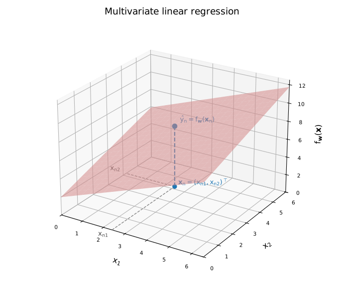
In an engineering example, \(x_1\) might be the load and \(x_2\) the temperature of a structural component. A linear model \(\hat y_n=w_0+w_1x_{n1}+w_2x_{n2}\) would assign one coefficient to each feature. Under this model specification, changing \(x_1\) while holding \(x_2\) fixed changes the prediction by \(w_1\) times the change in \(x_1\). This is a useful interpretation of a regression coefficient, but it is not automatically evidence of a causal effect of load or temperature on the observed quantity.
3.3 The augmented feature vector and the dot product
A small change in notation allows us to write the entire multivariate prediction compactly. We append a constant feature equal to \(1\) to every input vector and include the intercept among the weights:
\[ \tilde{\mathbf x}_n= \begin{bmatrix}1\\x_{n1}\\\vdots\\x_{nD}\end{bmatrix} \in\mathbb R^{D+1},\qquad \tilde{\mathbf w}= \begin{bmatrix}w_0\\w_1\\\vdots\\w_D\end{bmatrix} \in\mathbb R^{D+1}. \]
Multiplying the corresponding entries and summing gives exactly the original linear-regression equation:
\[ \boxed{\hat y_n=f_{\tilde{\mathbf w}}(\mathbf x_n) =\tilde{\mathbf x}_n^\top\tilde{\mathbf w} =w_0+\sum_{d=1}^{D}w_dx_{nd}.} \]
The leading \(1\) is not an observed physical measurement; it is an artificial constant feature introduced solely to absorb the intercept into the dot product. We use the tilde to distinguish augmented vectors from the original input vectors. This makes the mathematical notation convenient and permits the same computational operation to handle all coefficients, including \(w_0\).
Worked example. Suppose \(D=2\), \(\mathbf x_n=(2,3)^\top\), and the fitted parameters are \(w_0=4\), \(w_1=1.5\), and \(w_2=-2\). Then
\[ \tilde{\mathbf x}_n=\begin{bmatrix}1\\2\\3\end{bmatrix},\qquad \tilde{\mathbf w}=\begin{bmatrix}4\\1.5\\-2\end{bmatrix},\qquad \hat y_n=1(4)+2(1.5)+3(-2)=1. \]
The prediction is unchanged if we use the expanded expression or the compact dot product. The matrix and vector dimensions are compatible because both augmented vectors have \(D+1\) entries.
We can also augment the full dataset with a column of ones:
\[ \tilde X=\begin{bmatrix} 1&x_{11}&\cdots&x_{1D}\\ 1&x_{21}&\cdots&x_{2D}\\ \vdots&\vdots&\ddots&\vdots\\ 1&x_{N1}&\cdots&x_{ND} \end{bmatrix}\in\mathbb R^{N\times(D+1)}. \]
The predictions for all observations can then be computed simultaneously:
\[ \boxed{\hat{\mathbf y}=\tilde X\tilde{\mathbf w}\in\mathbb R^N.} \]
The dimensions explain why the product is valid: an \(N\times(D+1)\) matrix multiplied by a \((D+1)\times1\) vector produces an \(N\times1\) vector. Dot products and matrix multiplication are central computational operations in machine learning, and efficient hardware such as GPUs can perform many such operations rapidly.
4 Learning and fitting the model
Writing down a regression function is not the same as determining which function best matches the observations. The model family specifies the form of the relationship; the values of its parameters remain unknown. Given the pairs \((\mathbf x_n,y_n)\), we want to find coefficients \(\tilde{\mathbf w}\) that produce suitable predictions. This procedure is variously called learning, parameter estimation, or model fitting.
To judge a set of parameters, we need to examine how its predictions compare with the observed targets. The difference
\[ \boxed{e_n=y_n-\hat y_n} \]
is a residual for observation \(n\). A positive residual means the observed output exceeds the prediction; a negative residual means the model predicted a value larger than the observation. Residuals help us describe discrepancies but do not, by themselves, specify how all discrepancies should be combined into one measure of fit.
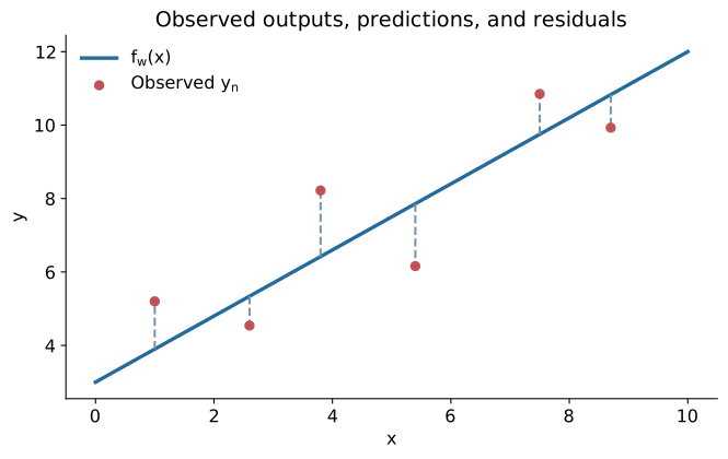
A loss function will provide a numerical way to quantify prediction errors across the dataset, and an optimization algorithm will provide a systematic way to search for parameter values with a smaller loss. A naive search could try many candidate coefficients and compare their predictions; more structured optimization procedures exploit the mathematical form of the objective to update parameters efficiently. For example, gradient-based methods use information about how the loss changes with the parameters. The formal definitions and derivations of loss functions and optimization are developed in subsequent chapters; here the key distinction is that computing predictions for fixed parameters is straightforward, while learning good parameters requires an additional criterion and method.
A small residual on training observations is not the only criterion of usefulness. We ultimately want predictions that remain reasonable on new observations. This relates the regression problem back to generalization, introduced in Chapter 1, and motivates studying both model complexity and available data.
4.1 Overparameterization and non-unique solutions
A simple example reveals an important difficulty. Suppose we have only one observed point \((x_1,y_1)\) and try to fit a line
\[ y_1=w_0+w_1x_1. \]
There is one equation but two unknowns, \(w_0\) and \(w_1\). For any chosen slope \(w_1\), we can set \(w_0=y_1-w_1x_1\) to obtain a line passing exactly through the observed point. Hence infinitely many different parameter pairs fit that single observation perfectly. The observed data do not uniquely determine the parameters.
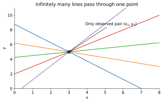
This is an example of an underdetermined problem: the available equations do not identify a unique solution. More generally, with \(D\) features and an intercept, a linear regression model contains \(D+1\) parameters. If the number of observations is smaller than the number of parameters (\(N<D+1\)), the augmented data matrix cannot have full column rank, and the parameters cannot be uniquely identified from the linear equations alone. The familiar shorthand \(D>N\) describes a strongly overparameterized regime, but the intercept should be counted when comparing the total number of parameters with the number of observations.
The number of observations and parameters is not the whole story. Even if \(N\ge D+1\), a unique fit may still be impossible if some columns of the data matrix are linearly dependent. Conversely, if the model cannot express the observed trend well, adding more data alone does not guarantee a good fit. What matters is both the available information and the expressive capacity of the chosen model.
An overparameterized model is not necessarily useless. In some modern machine-learning settings, models with very many parameters can still produce meaningful predictions. However, being able to fit the training data exactly does not imply that the chosen parameters will predict unseen observations accurately. Techniques such as regularization, together with model evaluation on unseen data, help control the solutions preferred during learning. The details of overfitting, regularization, and generalization will be studied later. This simple example is important because the same tension between model flexibility, parameter identifiability, and prediction on new cases appears far beyond straight-line regression.
4.2 Interactive Examples: Fitting Linear Regression Models
The following interactive examples illustrate how the parameters of linear regression models influence their predictions and their agreement with observed data. Both examples consider the prediction of concrete compressive strength using information about the concrete mixture.
The first example uses cement content as a single input variable, resulting in a regression line controlled by an intercept and a slope. The second example introduces water content as an additional input variable, producing a regression plane controlled by three parameters.
By adjusting these parameters, we can observe how the predicted values change and how closely the resulting line or plane fits the available observations. The vertical differences between the observed and predicted values are called residuals:
\(e_n=y_i-\hat y_n.\)
The animations also illustrate how prediction errors can be summarized using the mean squared error (MSE):
\(\mathrm{MSE}=\frac{1}{N}\sum_{n=1}^{N}(y_n-\hat y_n)^2.\)
The objective is not yet to derive an optimization algorithm, but to understand how model parameters, residuals, and fitting quality are related. These ideas provide the foundation for studying loss functions and optimization in greater detail.
5 Interpreting regression responsibly
5.1 Correlation Is Not Causation
Regression models are useful for identifying relationships between variables and making predictions from observed data. However, a statistical relationship does not necessarily imply that one variable causes changes in another. Two quantities may increase or decrease together because they are influenced by a common factor, share a similar trend over time, or simply exhibit a coincidental relationship.
This distinction is particularly important when interpreting regression models. For example, buildings with greater electricity consumption may also have higher maintenance costs. However, this does not necessarily mean that electricity consumption causes maintenance costs to increase. Larger buildings may simultaneously consume more electricity and require more maintenance because of their size, occupancy, and operational demands. In this case, building size may act as a confounding variable, influencing both quantities and contributing to the observed correlation.
Strong correlations can also arise between entirely unrelated variables. For example, historical records show correlations between UFO sightings in Hawaii and successful Mount Everest climbs, as well as between Disney movie releases and motor vehicle theft rates in the United States. Although these datasets exhibit remarkably similar trends, there is no plausible causal connection between the corresponding variables. Such examples demonstrate that even a strong correlation can be misleading when interpreted without considering the underlying context.
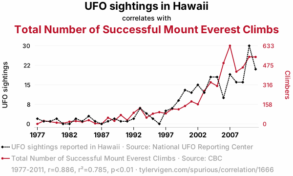
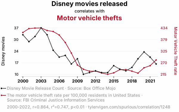
In scientific and engineering applications, predicting an outcome is different from explaining what causes it. A regression model may produce useful predictions without representing a causal relationship. Establishing causation requires additional evidence, careful consideration of confounding variables, appropriate study designs, and an understanding of the physical mechanisms involved. Regression results should therefore be interpreted alongside domain knowledge rather than treated as proof of causation.
5.2 Terminology across disciplines
The same quantities often have different names in machine learning, statistics, and applied research. An input variable may be called a feature, predictor, covariate, explanatory variable, independent variable, or regressor. An output variable may be called a target, response, outcome, dependent variable, or regressand. Some terms—particularly exogenous and endogenous—have more specific meanings in econometrics and should not be treated as perfect synonyms in every context. Throughout these notes, input/feature and output/target will be the default vocabulary.
5.3 Prediction, interpretation, and causal questions
It is helpful to distinguish what a scientific or engineering question is actually asking. “What is the expected life expectancy of someone with a given smoking history?” is a prediction question. “Does smoking cause cancer?” is a causal question: it asks what smoking itself changes, not merely what variables are associated in the observed sample. “How does expected life expectancy differ with cigarette consumption?” can be formulated as an association or interpretation question, but answering it causally would require further assumptions. Similarly, estimating the probability of a large earthquake within a future time window is a forecasting problem, whereas identifying why a particular structure failed is a different question involving physical mechanisms and causal evidence. A regression equation alone does not resolve these differences.
5.4 A model without an offset
In the linear regression models discussed so far, we have used (D+1) parameters to represent data with (D) input features. An alternative, sometimes used in practice for high-dimensional data, is to omit the intercept (or offset) term (w_0). The model then becomes
\[ \hat y_n=f_{\mathbf w}(\mathbf x_n) =w_1x_{n1}+\cdots+w_Dx_{nD} =\mathbf x_n^\top\mathbf w, \]
where \(\mathbf x_n\in\mathbb R^D\) and \(\mathbf w\in\mathbb R^D\).
In this case, the model has \(D\) parameters instead of \(D+1\). Without an intercept, the regression function passes through the origin, meaning that a zero input vector produces a prediction of zero. Whether this assumption is appropriate depends on the problem and the relationship being modelled.
Finally, it is important to distinguish between the number of input features and the number of model parameters. Although these quantities are closely related in linear regression, they can differ substantially for other machine learning models. For example, a neural network may contain many more trainable parameters than the number of features in its input.
5.5 Matrix multiplication: a short refresher
For matrices \(A\in\mathbb R^{M\times N}\) and \(B\in\mathbb R^{N\times D}\), the product \(AB\) is defined and satisfies
\[ \boxed{A_{M\times N}B_{N\times D}=C_{M\times D},\qquad C_{ij}=\sum_{k=1}^{N}A_{ik}B_{kj}.} \]
The inner dimensions must agree. If instead \(A\) had \(N_1\) columns and \(B\) had \(N_2\) rows, the product would be valid only when \(N_1=N_2\). This simple rule is worth checking whenever vectors and matrices are combined. In regression, the product \(\tilde X\tilde{\mathbf w}\) works precisely because the number of augmented features equals the number of parameter entries.
6 Chapter Summary
Regression provides a framework for relating one or more input variables to a numerical output. Its two main objectives are prediction, where we estimate outputs for new inputs, and interpretation, where we study relationships between variables. A regression dataset containing \(N\) observations and \(D\) input features can be represented by a data matrix \(X\in\mathbb R^{N\times D}\) and a target vector \(\mathbf y\in\mathbb R^N\). A regression function uses the input features to produce predictions that approximate the observed outputs.
Linear regression represents these predictions as a linear combination of input features. With one input, the model is a straight line, \(\hat y=w_0+w_1x\), where \(w_0\) is the intercept and \(w_1\) is the slope. With multiple inputs, the model generalizes to a plane or hyperplane. By introducing an augmented feature vector containing a constant \(1\), we can express the prediction as a dot product, \(\hat y_n=\tilde{\mathbf x}_n^\top\tilde{\mathbf w}\), and compute predictions for the entire dataset using \(\hat{\mathbf y}=\tilde X\tilde{\mathbf w}\).
Learning or fitting a regression model involves determining parameter values that produce suitable predictions from the available observations. The difference between an observed output and its prediction is called a residual, \(e_n=y_n-\hat y_n\). These differences can be summarized using a measure such as the mean squared error (MSE), which helps quantify how closely a model fits the data. Finding parameters that reduce prediction errors requires an optimization procedure, which will be studied in subsequent chapters.
An important challenge arises when a model contains more parameters than the available observations can uniquely determine. In such overparameterized or underdetermined problems, different parameter values may produce equally good fits to the training data. However, a good fit does not necessarily guarantee accurate predictions for unseen observations, highlighting the importance of generalization.
Finally, regression results must be interpreted responsibly. A statistical association does not establish causation, and apparent relationships may be influenced by confounding variables or coincidental trends. The choice of input features, inclusion of an intercept, and interpretation of model coefficients should therefore be guided by the application context and relevant domain knowledge.
6.1 Check Your Understanding
- What are the two main objectives of regression? Give one practical example of prediction and one of interpretation.
- What do \(N\), \(D\), \(x_{nd}\), \(\mathbf x_n\), \(X\), and \(\mathbf y\) represent in a regression dataset? Specify the dimensions of the vectors and matrices.
- Consider the dataset containing height, age, and weight presented in this chapter. How would the input matrix \(X\) change if age were excluded? Would the number of observations change?
- Write the equation of a univariate linear regression model: \[ \hat y_n=w_0+w_1x_n. \] Explain the meaning of the intercept \(w_0\) and slope \(w_1\), including their physical units.
- Write the prediction equation for a multivariate linear regression model with three input features and an intercept. How many parameters does the model contain?
- Why do we add a constant \(1\) to create an augmented feature vector? Explain how this allows a linear regression model to be expressed as a dot product: \[ \hat y_n=\tilde{\mathbf x}_n^\top\tilde{\mathbf w}. \] Verify the dimensions of the matrix-vector product: \[ \hat{\mathbf y}=\tilde X\tilde{\mathbf w}. \]
- Consider a linear regression model with two input features and the following parameters: \[ \mathbf x_n= \begin{bmatrix} 2\\ 3 \end{bmatrix}, \qquad w_0=4,\quad w_1=1.5,\quad w_2=-2. \] Calculate the predicted output using both the expanded equation and the augmented-vector representation.
- What is a residual in regression? Consider the expression: \[ e_n=y_n-\hat y_n. \] Explain what positive and negative residuals indicate.
- What is the mean squared error (MSE), and how does it help evaluate how well a regression model fits the observed data? \[ \mathrm{MSE} =\frac{1}{N}\sum_{n=1}^{N}(y_n-\hat y_n)^2. \] What happens to the MSE when the model parameters change?
- What does it mean to fit or estimate the parameters of a regression model? Why do we need a loss function and an optimization procedure?
- Suppose we have only one observation \((x_1,y_1)\) and want to fit a straight line: \[ y_1=w_0+w_1x_1. \] Explain why infinitely many lines can pass through that point. How does this relate to overparameterization?
- Why does a small training error, or even a perfect fit to the training observations, not guarantee accurate predictions for new inputs?
- What is the difference between correlation and causation? Give an example from engineering in which two variables may be correlated because they are influenced by a third variable.
- What happens when the intercept is removed from a linear regression model? \[ \hat y_n=\mathbf x_n^\top\mathbf w. \] How does this affect the number of parameters and the geometric interpretation of the regression function?
- Consider two matrices: \[ A\in\mathbb R^{M\times N}, \qquad B\in\mathbb R^{N\times D}. \] What are the dimensions of \(AB\), and what condition must be satisfied for matrix multiplication to be valid?
6.2 Coming next
The next chapter introduces loss functions, which turn differences between predictions and observed targets into a numerical criterion for comparing candidate models. We will then develop optimization methods for adjusting parameters systematically. These ideas make it possible to move from specifying a regression model to learning its parameters from data.
7 Acknowledgements and AI Disclosure
7.1 Acknowledgements
These lecture notes were developed with reference to the teaching materials of CS-433 Machine Learning, offered by the School of Computer and Communication Sciences at the École Polytechnique Fédérale de Lausanne (EPFL), Switzerland.
The original course provided a valuable reference for the selection, organization, and explanation of foundational machine learning concepts. The materials have been adapted, reorganized, and extended for the objectives of the present course, including additional examples and applications in civil engineering.
Reference course: EPFL CS-433 — Machine Learning.
This is an independent adaptation and does not imply endorsement by EPFL or the original course instructors.
7.2 Use of Generative AI
Generative AI tools were used to assist with drafting and editing lecture content, preparing examples, generating and refining figures, and developing interactive animations and visualizations.
The course instructor directed the development of these materials and remains responsible for their selection, organization, technical accuracy, and final presentation. AI-generated content was used as supporting material rather than as an independent authoritative source.
External figures, datasets, and other third-party materials are acknowledged separately where appropriate.